Predicting Application Workload via Extreme Value Analysis

Scalability plays a key role in the success of an application/service. Being able to remain responsive in the face of heavy loads is crucial for a growing application. A lot of effort is spent to design scalable systems with the aid of state of the art paradigms, frameworks and tools. Developing a scalable system is, however, only part of the solutions. A system capable of scaling is of no use if we do not know when to scale it. The point is that we want our services to scale up/out when the load is intensifying but at the same time we want to strongly avoid scaling up/out when not needed. Scaling, in fact, never comes for free: additional resources mean additional costs that we want to avoid if not really necessary.

To complicate this scenario, we might have committed to provide our users with a specific service level (e.g. through a Service Level Agreement). In this cases we can not afford to scale up/out when the load reaches critical levels but we rather want to be proactive. That is, we scale up/out before the Quality of Service offered to the users degrades. Proactiveness, however, often leads to provisioning and non cost-effective decisions.

I am currently working on a web application that does some heavy sound processing (as beat detection that I discussed here) on user-submitted audio files. I want the processing service to scale proactively without ever degrading user experience (avoid long wait times). I am able to scale out these services but I don’t want to waste money on unused resources so I was after some tool to aid me predict the load on my system to more accurately decide when to scale. Several tools allow engineers to monitor the resource consumption (CPU, memory, network) and load of their systems. Few techniques however are available to guide proactive scaling. Few tools, in fact, help engineers and system designers to quantify possible future peaks in their system’s workload. And almost none of such tools provides a quantifiable confidence on the predicted peak. Workload prediction (as well as resource demand prediction) is often performed by experts on the basis of time series and real-time information but is hardly guided by statistical/scientific evidence.

In this scenario, Extreme Value Analysis can help predicting workload peaks starting from time series and can therefore serve as a fruitful aid to proactive scaling.

Extreme Value Analysis

Extreme Value Analysis (EVA) is a statistical theory that aims at assessing the probability of extreme events given an ordered sample of a random variable. EVA is applied in several fields as for instance, structural engineering, finance and traffic prediction. Recent studies also apply EVA to the prediction of network congestions.

For practical applications of EVA, the Block Maxima technique can be used. With block maxima the input time series is divided into blocks of fixed size from each of which only the maximum value is taken. The resulting sample is called block maxima serer. EVA then fits to the block maxima data a Generalized Extreme Value (GEV) distribution. GEV distribution is a family of continuous distributions that approximates well the behaviour of maximum values in a time series.

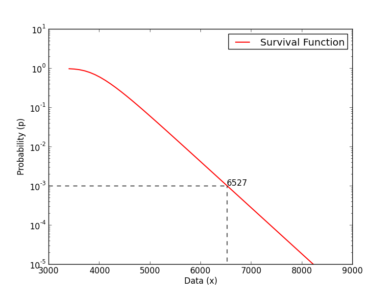
Once a GEV continuous distribution has been fit to the data a survival function can be extracted from it. The survival function (also known as reliability function or complementary cumulative distribution function) says for any value x, the probability p that a value higher than x occurs in the event represented by the original data. As you can understand with such a distribution we can choose a probability value p and extract the corresponding value x such that the probability of witnessing a value higher than x is p. That is, we can not only identify peaks but also quantify the probability of exceeding them.

In figure above an example of a survival function is shown. As you can see from the plot, the value 6527 is associated to the probability \(10^{-3}\) which means that, in the event represented by the input time series, the probability of observing values that exceed 6527 is only \(10^{-3}\).

Predicting Workload

In the context of predicting workload peaks, the time series fed to Extreme Value Analysis can represent either traffic load, memory consumption, CPU usage and so on. Consider for instance traffic load, but the same reasoning also applies to other metrics.

Given a time series representing traffic load we can apply EVA to that data. Extreme Value Analysis fits to the block maxima a GEV continuous distribution. From the corresponding survival function we are able to extract traffic values that are only exceeded with arbitrarily low probabilities.
For instance, let’s pick a probability \(p = 10^{-3}\) and its corresponding traffic load value x. We now not only have a prediction of future traffic load but also the probability that this prediction is exceeded. Scaling up/out our service so that is can handle the traffic load x means knowing that the probability of overloading the service is \(p = 10^{-3}\). That is, 99.9% of uptime.

Example

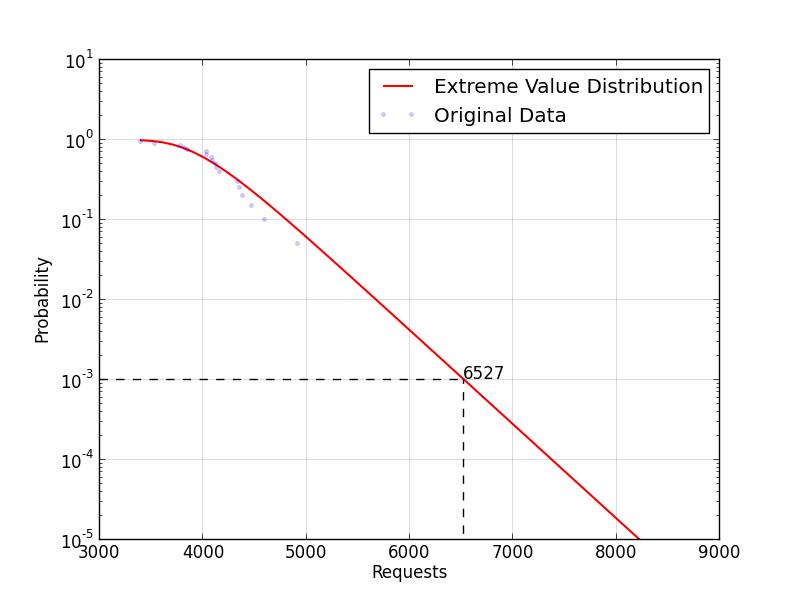
Consider as an example the following time series representing the maximum daily number of simultaneous requests to a service (for the last 20 days):

[ 4352, 4472, 3847, 4915, 4969, 4333, 4381, 4091, 4135, 4160,
3534, 4598, 4086, 3788, 4038, 3396, 4118, 3822, 4333, 4034 ]

If we apply Extreme Value Analysis to that data we get the following survival function:

Scaling out the service so that it can handle 6527 simultaneous requests ensures us that it will be overloaded only with a probability \(p = 10^{-3}\) which is a 99.9% daily uptime.

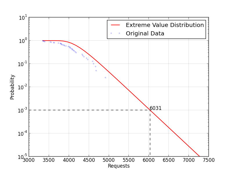
In addition, the more data we have, the more accurately we can predict possible peaks. If we extend the previous example data with other 20 values (for a total of 40 days):

[ 4352, 4472, 3847, 4915, 4969, 4333, 4381, 4091, 4135, 4160,
3534, 4598, 4086, 3788, 4038, 3396, 4118, 3822, 4333, 4034,
3738, 4670, 3346, 4070, 3556, 3810, 3984, 3892, 4615, 3634,
4016, 3378, 4441, 3800, 4182, 3879, 3926, 3625, 4687, 3366 ]

If we apply Extreme Value Analysis to that data we get the following survival function:

That associates to \(p = 10^{-3}\) a lower workload value (6031).

Source Code

You can find the Python pyscale module that implements the workload prediction on Github. To predict a load peak at a given probability you can instantiate an object of the class LoadPredictor as:

from pyscale import LoadPredictor

load_data = [ 4352, 4472, 3847, 4915, 4969, 4333, 4381, 4091, 4135, 4160,  
              3534, 4598, 4086, 3788, 4038, 3396, 4118, 3822, 4333, 4034 ]
predictor = LoadPredictor(load_data)
load_peak = predict_load(0.001)

You can also produce a plot of the survival function by instantiating an object of the class PredictionPlotter:

from pyscale import LoadPredictor

load_data = [ 4352, 4472, 3847, 4915, 4969, 4333, 4381, 4091, 4135, 4160,  
              3534, 4598, 4086, 3788, 4038, 3396, 4118, 3822, 4333, 4034 ]
predictor = LoadPredictor(load_data)
plotter   = PredictionPlotter(predictor)
plotter.xlabel('Requests')
plotter.ylabel('Probability')
plotter.plot("plot.png", 0.001)

Notes

I would like to compare the workloads predicted by this approach with real load data of a growing web service. That would allow me to really understand the cost impact of scaling when guided by these predictions. Unluckily, I don’t have real-word data for a thorough evaluation now but I should have them reasonably soon (as soon as I get those data I will update this post). If you ever give a try to this approach and collect some data from your services/applications please contact me as I would love to have a look at the results.